Malaysia’s Climate Finance: From Access to Delivery

Starting with the financing question

Malaysia’s ambition is substantial. The National Energy Transition Roadmap (NETR) estimates RM1.2–1.3 trillion of investment through 2050. That figure describes energy-transition investment, rather than an external financing gap. The World Bank’s 2026 Malaysia Country Climate and Development Report takes a broader view, covering incremental mitigation and adaptation investment over 2025–2050, including infrastructure retrofits. The two estimates answer different questions; adding them would obscure the scale each is intended to describe.¹, ²

Before asking how much of the national need a funding channel can meet, put both sides of the comparison on the same basis. They must cover compatible sectors and years, use consistent currency and price assumptions, and distinguish total investment from additional investment. They must also count finance at the same stage. An approved regional fund cannot be treated as money received by Malaysia.

The size of a contribution is only one part of its value. A relatively small amount of capital could help a viable project proceed if its terms address a risk that other investors cannot accept. To establish that effect, examine the actual terms, the alternatives available and the investment that follows. The presence of co-financing alone cannot show what the public contribution made possible.

Following the money through each stage

A regional programme shows why these distinctions matter. The Green Climate Fund (GCF) approved FP296, Navis Decarbonization Fund I, on 28 March 2026 for a programme targeting Indonesia, Malaysia, the Philippines and Thailand. Its published financing breakdown lists US$60 million of GCF equity and US$240 million of co-financing.³

The project record also lists a legal-opinion milestone on 15 July 2026. Together, these dated events establish progress through the programme’s approval process. They do not establish how much was allocated to Malaysia or whether a Malaysian investment received payment. The page’s inconsistent elapsed-day counter also limits its usefulness as a statement of current implementation status.³

A project owner therefore needs to look beyond the programme announcement. Does the project fit the investment mandate? Who decides whether to invest? What due diligence remains, and which conditions must be met before commitment and payment? Answers to those questions determine the work still ahead.

The same logic should shape institutional reporting. Record the amount requested, approved, committed and paid, with a date, an accountable party and evidence for each stage. Then follow the money into its intended use and measured results. The legal sequence may differ across transactions, but the distinction between a promise and a payment remains essential.

One further question deserves its own assessment: did the public contribution attract investment that would otherwise have stayed away? The co-financing shown in a programme’s structure cannot answer that. Establishing additional investment requires evidence about what financiers would have done without the support.

Making accreditation a portfolio decision

Once the potential projects and funding routes are clear, an institution can make a more useful decision about accreditation. Direct accreditation may build lasting capability and give it greater control over project origination. An existing accredited partner offers another route, with its own capabilities and constraints. The choice should turn on the work the institution expects to undertake.

For GCF, that comparison needs to reflect the framework effective from 31 October 2025, subject to transitional arrangements. It removes the fixed accreditation term. Operational guidance describes two application cycles a year and a nine-month review by the Secretariat and Accreditation Panel, excluding applicant response time. The nine months cover that review stage; they do not predict the total time to accreditation, project approval or payment.⁵, ⁶, ⁷

Past experience still matters, but it needs careful interpretation. An accredited entity without an approved project may be unsuccessful, still preparing a proposal or awaiting a decision. A snapshot cannot tell us which. Comparing routes requires histories that include pending, rejected and withdrawn cases, with enough follow-up to understand what happened.

Before committing substantial resources, ask three questions. Is there a credible pipeline that will use the capability repeatedly? How does the full cost of building and maintaining it compare with a partner’s fees and constraints? And what additional control or project coverage would direct accreditation provide? Include fiduciary duties, safeguards and monitoring in that assessment; the responsibilities continue after access has been secured.

The answer need not be an exclusive choice. An institution with recurring demand and suitable capability may pursue direct accreditation while selected projects proceed through partners. A smaller or uncertain pipeline may justify starting with a partnership. The evidence reviewed here does not establish which route would be faster or cheaper for a particular Malaysian institution.

Eligibility also needs to be checked fund by fund. GCF’s governing instrument makes developing-country Parties eligible and does not specify automatic exclusion at the World Bank’s high-income threshold. Other programmes have their own rules, and income may affect their terms or allocation decisions.⁸

Making preparation count

An access route is valuable only if there are projects ready to use it. Preparation should therefore have a specific job: resolve an uncertainty or requirement that stands in the way of an investment decision. More studies and better documents are useful when they change what a financier can confidently assess.

Malaysia’s Climate Finance Innovation Lab (CFIL) offers a useful starting point for examining that progress. In its account dated 30 July 2026, Bank Pembangunan Malaysia Berhad (BPMB) reported 23 projects in the inaugural cohort seeking approximately RM3.47 billion, with 15 participating in the accelerator. One project subsequently secured an international grant. The announcement does not disclose the amount, payment status or how much the programme contributed to the outcome.⁹

The next cohort provides another opportunity to learn. A joint statement from Bank Negara Malaysia and the Securities Commission on 13 August 2026 reported 22 projects seeking RM1.73 billion, with accelerator support planned. That is a measure of demand in a selected pipeline. Tracking what happens next would turn it into a more useful account of financing progress.⁴

Programme managers can begin before support starts. For each project, record the finance sought, offers already available, unresolved requirements, responsible owner and development stage. Then track the support provided and the investor’s response. A project that proceeds, stalls or withdraws should leave a record of why, so the next round of preparation can address what actually matters.

Those records would improve management immediately and provide a basis for evaluating impact. A credible evaluation would also compare suitable projects, account for selection and follow-up, and examine the experience of applicants and financiers. The documentary evidence used here cannot establish preparation’s effect; the reported grant should not be converted into a programme success rate.

Matching capital to the constraint

Preparation may reveal a problem that better documentation cannot solve. A project could lack a dependable repayment source, expose investors to a risk they cannot hold, or create public benefits without enough revenue from users. Each requires a different financing response.

NETR distinguishes commercially viable projects from those needing additional financing support. The World Bank’s 2026 report also points to a combination of public resources, domestic private participation and external finance, while highlighting the challenge of bankability. These diagnoses support considering several instruments. The project’s economics must determine which combination is appropriate.¹, ²

The evidence a financier needs should be equally specific. Measurement, reporting and verification (MRV) can serve a lender’s emissions covenant, a fund’s climate-impact assessment or a national carbon-pricing system. These purposes do not necessarily require the same data or authority. Before commissioning more work, establish what must be demonstrated and who can accept the evidence.

In a parliamentary answer dated 12 March 2026, Malaysia’s environment ministry described MRV as a foundation for planned carbon-pricing instruments. That statement does not make one national law a prerequisite for all commercial climate finance. This analysis does not establish subsequent enactment or commencement; where a transaction depends on a legal change, its status must be checked against the specific requirement.¹⁰

Stress-testing the financing structure

Choosing an instrument is only the beginning. The next question is whether the project can meet its obligations when cash flow disappoints. Consider a hypothetical RM100m project funded by RM70m of debt and RM30m of equity. Its reference annual cash available for debt service (CFADS) is RM15m, after operating expenses, taxes and required operating investment but before loan payments. These inputs are illustrative assumptions, not observations of a Malaysian project.¹¹

Compare two ways of financing the same project. The first uses RM70m of commercial debt at 7% over ten years. The second combines RM50m on those terms with RM20m at 3% over fifteen years. Both use fixed rates and fully amortising annual payments, with the first payment after one year and no grace period or balloon. The cheaper, longer loan replaces part of the commercial debt; it supplies no additional upfront capital.

During years 1–10, the mixed structure reduces annual debt service from RM9.97m to RM8.79m. Dividing CFADS by the scheduled payment gives the debt-service coverage ratio (DSCR). At 1.0, cash just covers the payment. We use 1.2 as an illustrative coverage requirement, allowing a margin above scheduled debt service; it is not a universal lender covenant.¹¹

The difference becomes clearer under stress. If cash flow falls by 40%, the commercial structure has a RM0.97m cash shortfall. The mixed structure can still make its payment, but only RM0.21m remains. Both fall below the 1.2 coverage requirement. Better financing terms provide breathing room while leaving the underlying operating risk in place.¹¹

A decision-maker can turn that result into a practical threshold. Maintaining coverage of 1.2 requires annual CFADS of RM11.96m under the commercial structure or RM10.55m under the mixed structure. Against the RM15m reference, those levels allow declines of 20.3% and 29.6%, respectively. The question for the project team is whether the remaining margin is adequate for the risks it faces.¹¹

Testing the probability assumptions

Stress scenarios show what happens at selected points. Simulation asks how often an outcome occurs within a specified set of assumptions. For each of three cash-flow distributions, we simulate 100,000 outcomes for a representative year during years 1–10. Both financing structures receive the same cash-flow shock in each draw, so the comparison isolates the effect of their payment schedules.¹¹

In every distribution, annual CFADS equals RM15m multiplied by X, which ranges from 0.55 to 1.15. Distribution A is triangular, with its most likely value at 1.00; B is triangular, with its most likely value at 0.85; C is uniform, giving equal probability density across the range. These choices produce mean annual cash flows of RM13.50m for A and RM12.75m for B and C. The RM15m reference is therefore not the expected cash flow. Comparing B with C changes the distribution’s shape while holding its range and mean constant; comparisons with A also change the mean.¹¹

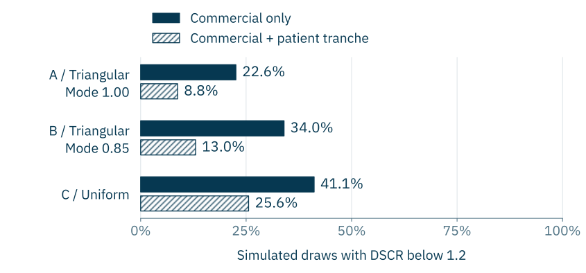
Source: Andi illustrative model SIM01; 100,000 draws per distribution, seed 20260908, common inverse-CDF random draws. One-year conditional frequencies, not empirical default probabilities or policy confidence.¹¹

The mixed structure has fewer outcomes below the coverage requirement in all three cases, as its lower scheduled payment would suggest. But the size of the estimated risk changes considerably with the distribution. Running more draws makes the calculation more precise; it cannot tell us which assumptions describe a real project.

That is the value of testing several assumptions. It shows both what the financing structure changes and how much the risk estimate depends on the view of cash flow. For an actual financing decision, replace the illustrative inputs with project records, revenue contracts, operating obligations and lender terms. Where evidence is incomplete, document expert judgments and test shared sources of downside risk. The example does not determine the availability or appropriate subsidy cost of patient capital.

Measuring the shortfall and the debt tail

The chance of a shortfall is only half the question. Its size matters too. The exhibit pairs the simulated frequency of cash falling below scheduled debt service with the average cash shortfall in the 5,000 draws with the lowest cash flow. Any zero shortfalls in that group remain in the average. This measures the project’s cash gap, rather than the lender’s eventual loss after recoveries.¹¹

There is also a trade-off beyond the first decade. Commercial debt is fully repaid by year 10, while the mixed structure still has RM7.67m of principal outstanding and requires annual payments of RM1.68m in years 11–15. Lower near-term payments leave obligations for later. The simulation covers a representative year, not a sequence of cash flows over the project’s life, so its frequencies cannot be compounded into lifetime default probabilities.¹¹

To make the calculation reproducible, the simulation uses Python’s Mersenne Twister, inverse-CDF transforms and a common random stream across the three distributions. Simulated threshold frequencies were checked against the exact distribution at τD/15, with τ equal to 1.0 or 1.2. Payment schedules and cash-shortfall calculations were checked separately.

Before using such a model for a financing commitment, extend it to the risks and terms of the actual transaction. This illustration excludes construction delays, fees, reserve accounts, remedies, refinancing, and uncertain interest rates or exchange rates. It also assumes patient capital is available and does not value its public subsidy cost. Those omissions matter to the final choice, even though the model is sufficient to show how repayment terms affect coverage.

Developing a practical decision agenda

These findings suggest a practical starting point for Malaysian institutions: take a manageable group of projects and connect each development expense to a financing decision. A definitive national ranking of obstacles is not needed to begin. What is needed is an accountable owner, a clear next step and evidence that will show whether the step was worthwhile.

The resulting record should be allowed to change the strategy. If well-prepared, otherwise viable projects repeatedly stall at an access requirement, invest in the relevant route or capability. If suitable financiers keep asking for the same missing evidence, improve preparation. If projects remain financially unviable despite good preparation, reconsider their capital structure, the public contribution or the project itself.

Interpret progress in the context of the projects selected. A more difficult cohort may move slowly even when support improves; an easier cohort may produce more approvals without better support. Reviewing costs, delays and unsuccessful cases alongside completed deals will make the next allocation of development effort better informed.

For the board, the immediate decision is where to commit the next increment of time and money, why it should help, and what would warrant a change of course. A climate-finance strategy becomes useful when it can answer those questions for the projects it is meant to serve.